Salary prediction using supervised learning
It was raining outside last Saturday and my plan to hike Mt.Takao was not happening. So this blog happened after I decided to spend the next 4 hours on a quick data challenge. The goal is to develop a salary prediction system based on existing data to provide salary estimates for new job postings. We are given a training dataset with 1 million data points (features + salaries) and also a test dataset with another 1 million data points (features only) for which we need to predict the salaries. In this post I will walk through the supervised learning workflow for building a predictive model for this problem. The source code is available here.
Data preparation
First I carried out exploratory data analysis to see if there is any information in the dataset that could drive model selection. Exploratory data analysis showed there were 5 observations with 0 as salary value. They were discarded. No duplicates (or mistyped values showing up as two different values), no missing values were found. We get down to analysing the data distribution.
Preliminary data analysis :
- The salary data is uniformly distributed across industries and job types.
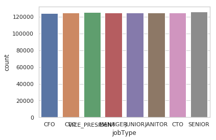
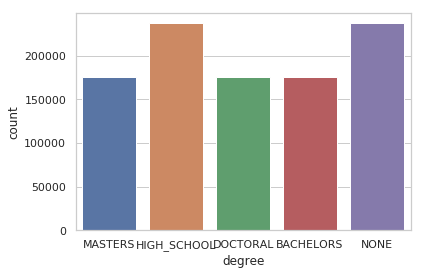
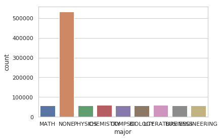
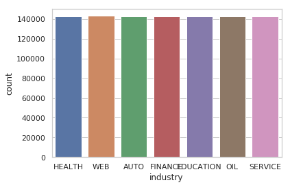
Figure 1: Distribution of salary data across categories
-
It is also almost evenly distributed across different degrees except for a large number of people about 47% who belong to either NONE or HIGH SCHOOL education levels.
-
Further, this could explain the fact that about 53% data has NONE as major. Which means there is no information about the major for ~6% whose majors is marked as NONE even though they have a BACHELORS or a higher level of education.
-
The distribution of the salaries follows the normal distribution.
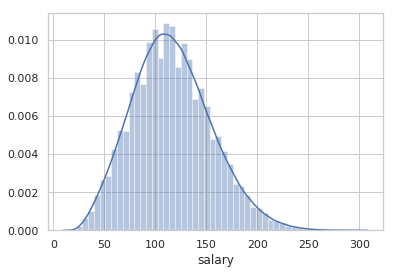
Figure 2: Distribution of all the salaries
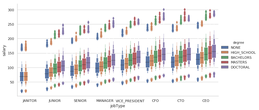
- Exploratory data analysis showed the relationship between the independent variables and the dependent variable ‘salary’ is generally linear.
#Check how degree and jobType combination varies with salary
degree_data = train_data.groupby(['jobType','degree']).mean().reset_index()
sns.catplot(x='jobType', y='salary', hue='degree', data=train_data.sort_values(['salary']), kind='boxen',aspect=2)
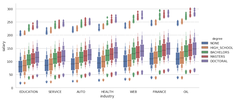
#Salary vs degree, in each industry
sns.catplot(x='industry', y='salary', hue='degree', data=train_data.sort_values(['salary']), kind='boxen',aspect=2)
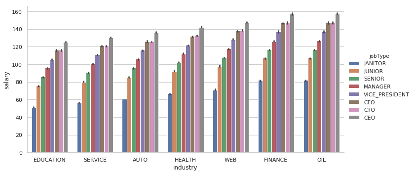
#Check how salary varies w.r.t. roles in each industry
sns.catplot(x='industry', y='salary', data=train_data.sort_values(['salary']), kind='bar', hue='jobType', estimator = np.median, aspect=2)
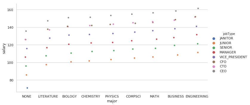
#Mean salary for different majors and job types (higher degrees have missing majors marked as NONE)
major_data = train_data[train_data['major']!='NONE']
major_data = pd.concat([major_data, train_data.loc[(train_data['major']=='NONE') & (train_data['degree'].isin(['HIGH_SCHOOL']))]])
major_data = major_data.groupby(['jobType','major']).mean().reset_index()
sns.catplot(x='major', y='salary', aspect = 2, hue='jobType', data=major_data.sort_values(['salary']))
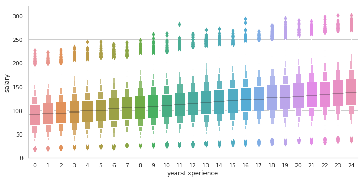
#Check how salary changes with experience
sns.catplot(x='yearsExperience', y='salary', data=train_data.sort_values(['salary']), kind='boxen', aspect=2)
#Check whether the relationship between salary and milesFromMetropolis is linear
sns.lineplot(x='milesFromMetropolis', y='salary', data=train_data.sort_values(['salary']))
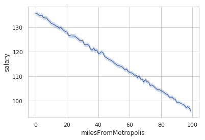
Figure 3: Linear relationship between different combinations of predictor variables and salary
These insights coupled with the fact that the training set has good coverage, with number of observations » number of attributes, indicates conventional linear regression is an appropriate starting point before going for ensemble methods like gradient boosting regression. These above mentioned observations would also mean regularization approaches like Lasso, Elastic Net or Ridge regression may not be required. To improve on the baseline performance of linear regression, I considered random forest regression and gradient boosting regression.
Regression
Linear regression works by modelling the relationship between the independent variables and the dependent variables by fitting a linear equation that is linear in the coefficients of the predictor variables.
Gradient boosting is an ensemble model which builds on shortcomings of an existing model in a sequential manner by fitting a regression tree which reduces the errors in residuals at each stage. We interpret the residuals as negative gradients and iterate until convergence. I use least squares regression for the the loss function (I couldn’t find any outliers in the data so least squares regression is good enough). The initial model here is based on calculating the mean of the salary values.
Preprocessing
I tried transforming the categorical variables —DEGREE, MAJOR, JOB_TYPE, INDUSTRY— into ordinal variables by ranking them. Transforming, first all of them at the same time, next only some of them, then different combinations of them. But as the results did not get better I stuck to the more general one-hot encoding.
import pandas as pd
predictor_copy = train_data.copy()
predictor_copy = pd.get_dummies(predictor_copy, columns=['jobType','degree','major','industry'], prefix=['jobType','degree','major','industry'])
Feature selection
From the exploratory data analysis, it was evident ‘milesFromMetropolis’ and ‘yearsExperience’ are linearly correlated with salary. Next to these variables, the type of the INDUSTRY had a huge impact as can be gleaned from the variable importance metric from the gradient boost regression algorithm.
Variable importance was derived by the calculating the amount by which each attribute variable split point improves the error for each of the regression trees in the gradient boosting algorithm. These values are then averaged for all the regression trees. There is a distinct linear relationship between the ‘jobType’ and DEGREE variables as well.
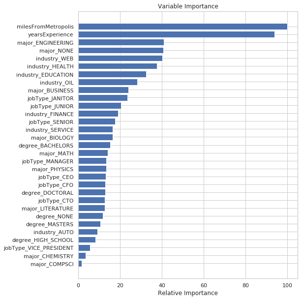
Figure 4: Variable importances output by the gradient boosting regression algorithm
From the exploratory data analysis, it was also clear that the 63 companies ‘companyId’ had least impact on salary. So I did not include the company information for training.
#Check how salary for a given job type varies with companyId
sns.catplot(data=train_data.groupby(['companyId','jobType']).mean().reset_index().sort_values(['salary']), x='jobType', y='salary', aspect=2)
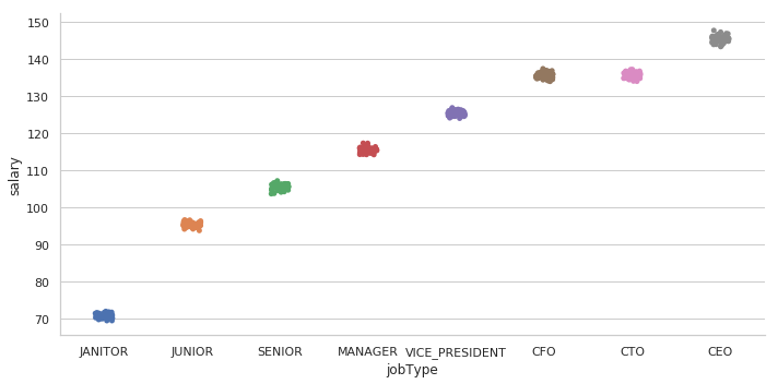
Figure 5: Mean salaries of different job types in every company
from sklearn.model_selection import train_test_split
X, y = predictor_copy.drop(['jobId','companyId','salary'],axis=1), predictor_copy['salary']
X_train, X_test, y_train, y_test = train_test_split(X, y, random_state=42)
Training
For training, the dataset had to be standardized with 0 mean and unit standard deviation for all the numeric variables to avoid a variable with huge variance dominating the model.
from sklearn.preprocessing import StandardScaler
scaler = StandardScaler()
X_train_std = scaler.fit_transform(X_train)
X_test_std = scaler.transform(X_test)
Since the number of features is small, overfitting is not a major concern here. Hence I did not use any regularization. For gradient boosting regression, I used least squares regression for the loss function as there were no outliers in the dataset when the numeric features were compared.
from sklearn.ensemble import GradientBoostingRegressor
gbr_model = GradientBoostingRegressor(n_estimators=500, random_state=42)
Validation
For validating our machine learning model, we repeatedly compare our model predictions against different subsets of the data marked for validation (25% of the observations) while training our model on all other data (75%) except the validation data. In my k(5)-fold cross validation setting, the values predicted by the machine-learning model and the ground-truth validation data are compared. RMSE is the square root of the mean squared errors (differences between predicted and observed values).
from sklearn.model_selection import cross_val_score
def rmse_cv(model):
    rmse = np.sqrt(-cross_val_score(model, X_train, y_train, scoring = 'neg_mean_squared_error', cv = 5))
    return(rmse)

cv_GBR=rmse_cv(model=gbr_model).mean()
- RMSE for Gradient Boosted Regression on the test dataset : 18.8632
Besides RMSE which penalizes big deviations by squaring them, one can also consider mean absolute deviations or MAE.
Programming language and libraries used
Python, scikit-learn for machine learning algorithms, matplotlib and seaborn for visualization, pandas for numerical analysis.